Topic 10: Image Processing
When remote sensing data are available in digital format, digital processing and analysis may be performed using a computer. Digital processing may be used to enhance data as a prelude to visual interpretation. Digital processing and analysis may also be carried out to automatically identify targets and extract information completely without manual intervention by a human interpreter.
Analog Images: remote sensing products such as aerial photos are the result of photographic imaging systems (i.e. Camera). Once the film is developed, then no more processing is required. In this case, the image data is refered to as being in an analog format.
Digital Images: remote sensed images can also be represented in a computer as arrays of pixels (picture elements), with each pixel corresponding to a digital number, representing the brightness level of that pixel in the image. In this case, the data are in a digital format. These types of digital images are referred to as raster images in which the pixels are arranged in rows and columns.
![]()
Pixel Values: The magnitude of the electromagnetic energy captured in a digital image is represented by positive digital numbers. The digital numbers are in the form of binary digits (or 'bits') which vary from 0 to a selected power of 2.
Each bit records an exponent of power 2 (e.g. 1 bit = 21 = 2). The maximum
number of brightness levels available depends on the number of bits used in representing
the energy recorded. Thus, if a sensor used 8 bits to record the data, there would be 28
= 256 digital values available, ranging from 0 to 255; 8-bit is the most common bit value.
| Image Type | Pixel Value | Color Levels |
| 8-bit image | 28 = 256 | 0-255 |
| 16-bit image | 216 = 65536 | 0-65535 |
| 24-bit image | 224 = 16777216 | 0-16777215 |
Image Resolution: the resolution of a digital image is dependant on the range in magnitude (i.e. range in brightness) of the pixel value. With a 2-bit image the maximum range in brightness is 22 = 4 values ranging from 0 to 3, resulting in a low resolution image. In an 8-bit image the maximum range in brightness is 28 = 256 values ranging from 0 to 255, which is a higher resolution image.
2-bit Image |
8-bit Image |
 |
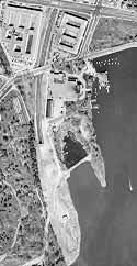 |
Image Restoration: most recorded images are subject to distortion due to noise which degrades the image. Two of the more common errors that occur in multi-spectral imagery are striping (or banding) and line dropouts.
Stripping or banding are errors that occur in the sensor response and/or data recording and transmission and results in a systematic error or shift of pixels between rows.
Dropped Lines are errors that occur in the sensor response and/or data recording and transmission which loses a row of pixels in the image.
One of the strengths of image processing is that it gives us the ability to enhance the view of an area by manipulating the pixel values, thus making it easier for visual interpretation. There are several techniques which we can use to enhance an image, such as Contrast Stretching and Spatial Filtering.
Image Histogram: For every digital image the pixel value represents the magnitude of an observed characteristic such as brightness level. An image histogram is a graphical representation of the brightness values that comprise an image. The brightness values (i.e. 0-255) are displayed along the x-axis of the graph. The frequency of occurrence of each of these values in the image is shown on the y-axis.
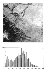 |
8-bit image (0 - 255 brightness levels) |
| Image Histogram x-axis = 0 to 255 y-axis = number of pixels |
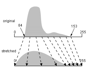
Contrast Stretching: Quite often the useful data in a digital image populates only a small portion of the available range of digital values (commonly 8 bits or 256 levels). Contrast enhancement involves changing the original values so that more of the available range is used, this then increases the contrast between features and their backgrounds. There are several types of contrast enhancements which can be subdivided into Linear and Non-Linear procedures.
Linear Contrast Stretch: This involves identifying lower and upper bounds from the histogram (usually the minimum and maximum brightness values in the image) and applying a transformation to stretch this range to fill the full range.
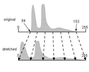
Equalized Contrast Stretch: This stretch assigns more display values (range) to the frequently occurring portions of the histogram. In this way, the detail in these areas will be better enhanced relative to those areas of the original histogram where values occur less frequently.
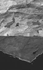
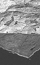
Linear Stretch Example: The linear contrast stretch enhances the contrast in the image with light toned areas appearing lighter and dark areas appearing darker, making visual interpretation much easier. This example illustrates the increase in contrast in an image before (left) and after (right) a linear contrast stretch.
Before Linear Stretch |
After Linear Stretch |
 |
 |
Spatial filters are designed to highlight or supress features in an image based on their spatial frequency. The spatial frequency is related to the textural characteristics of an image. Rapid variations in brightness levels ('roughness') reflect a high spatial frequency; 'smooth' areas with little variation in brightness level or tone are characterized by a low spatial frequency. Spatial filters are used to suppress 'noise' in an image, or to highlight specific image characteristics.
Low-pass Filters: These are used to emphasize large homogenous areas of similar tone and reduce the smaller detail. Low frequency areas are retained in the image resulting in a smoother appearance to the image.
Linear Stretched Image |
Low-pass Filter Image |
|
|
High-pass Filters: allow high frequency areas to pass with the resulting image having greater detail resulting in a sharpened image.
Linear Contrast Stretch |
Hi-pass Filter |
 |
 |
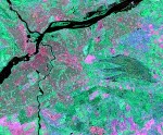
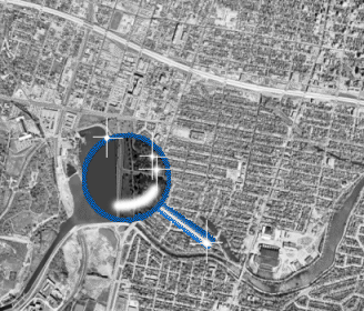
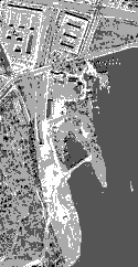
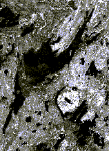
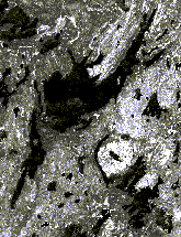
Directional Filters: are designed to enhance linear features such as roads, streams, faults, etc.The filters can be designed to enhance features which are oriented in specific directions, making these useful for radar imagery and for geological applications. Directional filters are also known as edge detection filters.
 |
 |
Edge Detection Lakes & Streams |
| Edge Detection Fractures & Shoreline |
||
Density Slicing: is a form of enhancement where the grey tones in an image are divided into a number of intervals reflecting a range of digital numbers. This transforms the image from a continuum of gray tones into a limited number of gray or color tones reflecting the specified ranges in digital numbers. This is useful in displaying weather satellite information (i.e. GOES Infrared maps):
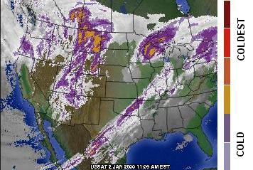 |
GOES Satellite infrared data is subdivided into 6 color levels from cold (white,gray, purple) to coldest (brown, red, dark brown). (from: The Weather Channel) |
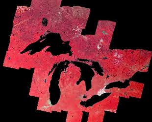
Mosaicing of Multiple Images: Images taken at different times and lighting conditions can be manipulated in order to produce a seamless mosaic from several images. In areas which are frequently cloud covered, it is possible to collect a number of images over time and selectively use only the portions which are nearly cloud-free in order to produce a cloud-free image mosaic of an area.
Great Lakes multiple image mosaic |
|
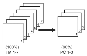
Satellite images obtained by remote sensing capture electromagnetic energy (i.e. light) by sampling over predetermined wavelength ranges which are refered to as 'bands' i.e. blue, green, red, near-infrared, mid-infrared, far-infrared, thermal infrared. In satellite sensors such as LANDSAT TM there are seven bands and these are represented as images of the earth for each of the wavelength ranges.
It is possible to extract additional information from digital images through a number of image processing techniques such as: False Color Composites, Image Ratios, and Principle Components Analysis, . The intent of these procedures is to make it easier for the image analyst to intepret the area or phenomenon being studied.
False Color Composites: LandSat TM produces 7 digital images of a scene representing the 7 bands of electromagnetic energy captured. These images can be processed individually as noted previously to enhance the image, but they remain grey-level images of the scene. It is possible to colorize a scene by applying a color to a selected band so that for example: Band 1 = Blue, Band 2 = Green, and Band 3 = Red. This produces a 'False Color' image of the scene.
Band 1 |
Band 2 |
Band 3 |
 |
 |
 |
False Color Composite |
||
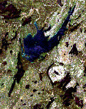 |
Image Ratios: It is possible to divide the digital numbers of one image band by those of another image band to create a third image. Ratio images may be used to remove the influence of light and shadow on a ridge due to the sun angle. It is also possible to calculate certain indices which can enhance vegetation or geology.
| Sensor | Image Ratio | EM Spectrum | Application |
| Landsat TM | Bands 3/2 | red/green | Soils |
| Landsat TM | Bands 4/3 | PhotoIR/red | Biomass |
| Landsat TM | Bands 7/5 | SWIR/NIR | Clay Minerals/Rock Alteration |
Normalized Difference Vegetation Index (NDVI): This is a commonly use vegetation index which uses the red and infrared bands of the EM spectrum.
NDVI = 100 * Square Root [(Red-IR)/(Red+IR)]
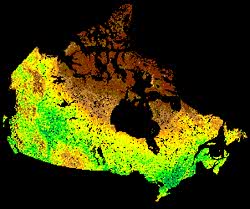 |
NDVI image of Canada. Green/Yellow/Brown represent decreasing magnitude of the vegetation index. |
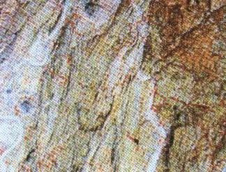
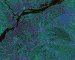
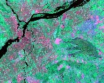
Principle Components Analysis: Different bands in multispectral images like those from Landsat TM have similar visual appearances since reflectances for the same surface cover types are almost equal. Principle Components Analysis is a statistical procedure designed to reduce the data redundancy and put as much information from the image bands into fewest number of components. The intent of the procedure is to produce an image which is easier to interpret than the original.
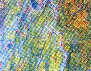
False color image with contrast stretch (SPOT data) |
PCA decorrelation stretch of same image |
|
|
In classifying features in an image we use the elements of visual interpretation to identify homogeneous groups of pixels which represent various features or land cover classes of interest. In digital images it is possible to model this process, to some extent, by using two methods: Unsupervised Classifications and Supervised Classifications.
Unsupervised Classifications: this is a computerized method without direction from the analyst in which pixels with similar digital numbers are grouped together into spectral classes using statistical procedures such as nearest neighbour and cluster analysis. The resulting image may then be interpreted by comparing the clusters produced with maps, airphotos, and other materials related to the image site.
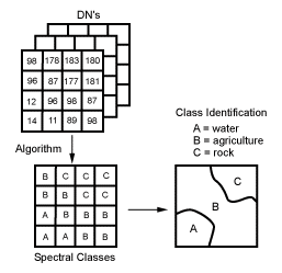
Supervised Classification: In a supervised classification the analyst identifies several areas in an image which represent know features or land cover. These known areas are refered to as 'training sites' where groups of pixels are a good representation of the land cover or surface phenomenon. Using the pixel information the computer program (algorithm) then looks for other areas which have a similar grouping and pixel value. The analyst decides on the training sites and thus supervises the classification process.
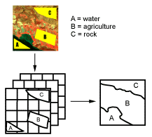
Limitations to Image Classification: Interpretation of classified images using supervised and unsupervised methods have to be approached with caution because it is a complex process with many assumptions. In supervised classifications, training areas may not have unique spectral characteristics resulting in incorrect classification. Unsupervised classifications may require field checking in order to identify spectral classes if they cannot be verified by other means (i.e. maps and airphotos).